I thought I understood LDA, until I learned this

Sometimes you think you understand a basic statistics problem. And then, you look closer and realize that you don’t understand it as well as you thought. This happened to me recently with Linear Discriminant Analysis (LDA). In this post, I discuss some interesting and lesser known aspects of LDA that I learned when diving deeper into this method, and that seem to often cause confusion.

Some of the lesser known facts about LDA that we will discuss here are:

• LDA refers to both a linear classifier and a separate dimensionality reduction method (our focus here)
• The dimensionality reduction method has a well known intuition, but different mathematical objectives are often used for this objective
• Some of the different mathematical objectives are equivalent, but others are not
• We prove that the LDA features are the eigenvectors of the matrix \(\mathbf{W}_{\mathbf{x}}^{-1} \mathbf{B}_{\mathbf{x}}\) where \(\mathbf{W}_{\mathbf{x}}\) is the within-class scatter matrix and \(\mathbf{B}_{\mathbf{x}}\) is the between-class scatter matrix
• LDA eigenvector features whiten the within-class covariance and diagonalize the between-class covariance
• LDA features do not necessarily maximize the performance of the LDA classifier

What is LDA? A tale of two methods

This first question can already be a source for confusion. The term LDA is commonly used to refer to two different but related techniques: 1) A linear classifier, and 2) a supervised dimensionality reduction method. This post is about the dimensionality reduction method, but it will be useful to first outline the classifier.

For both methods we will assume that we have a labeled dataset, with data vectors \(\{\mathbf{x}_1, \ldots, \mathbf{x}_N\}\) and labels \(\{y_1, \ldots, y_N\}\), with each \(\mathbf{x}_q \in \mathbb{R}^n\) and each \(y_q \in \{1, \ldots, c\}\). Here, \(N\) is the number of data points, \(n\) the dimensionality, and \(c\) is the number of classes.

The LDA classifier

The LDA classifier (how we’ll refer to this version of LDA onwards) is theoretically simple. It makes two essential assumptions:

1. That the distribution of the data conditional on the classes is Gaussian.
2. That all the classes have the same covariance (homoscedasticity)

In mathematical terms, LDA assumes that \(p(\mathbf{x}|y=k) = \mathcal{N}(\bar{\mathbf{x}}_k, \mathbf{W}_{\mathbf{x}})\), where \(\bar{\mathbf{x}}_k\) is the mean of the class \(i\), and \(\mathbf{W}_{\mathbf{x}}\) is the covariance matrix within each class, that is the same for all classes (this choice of notation will come handy later).

Under this assumption, the LDA classifier estimates the labels of new observations \(\mathbf{x}_q\) by computing the likelihoods \(p(\mathbf{x}_q|y=k)\) for each class, possibly combining them with a prior \(p(y=k)\), and then selecting the class with the highest likelihood or posterior probability. If all classes have the same priors, the estimated class is the one whose mean \(\bar{\mathbf{x}}_k\) is closest (in terms of the Mahalanobis distance) to the observations \(\mathbf{x}_q\). Because of the homoscedasticity assumption, this procedure leads to linear decision boundaries between the classes.

For the LDA classifier, only a subspace of the data matters

The LDA classifier has an interesting geometric implication for the data. In the \(n\)-dimensional space of the data, the class means \(\{\bar{\mathbf{x}}_1, \ldots, \bar{\mathbf{x}}_c\}\) will lie in a subspace of at most \(c-1\) dimensions. As we mentioned, for a given observation \(\mathbf{x}_q\), the LDA classifier will estimate the class by finding the closest class mean \(\bar{\mathbf{x}}_k\). Geometrically, the only relevant information for the LDA classifier is the projection of the data onto the subspace spanned by the means. The component of the data orthogonal to this subspace will not affect the classifier output, because they do not change what mean is closest to \(\mathbf{x}_q\).

Therefore, the LDA classifier implies a dimensionality reduction from \(n\) to \(c-1\) dimensions. This is not the same as the LDA dimensionality reduction method, however, as we will see next.

LDA dimensionality reduction: The intuition

We’ll refer to the LDA dimensionality reduction method as LDA-DR.

So, how is LDA-DR different from the dimensionality reduction implied by the LDA classifier? For this it is useful to consider some limitations of the dimensionality reduction implied by the LDA classifier:

1. The LDA classifier provides a \(c-1\) dimensional subspace, but we sometimes want to have a lower number of dimensions \(m < c-1\)
2. The LDA classifier does not provide specific filters that can be analyzed
3. The LDA classifier does not provide an ordering of the reduced space dimensions by relevance

The LDA-DR method addresses these limitations by providing a method for learning an \(m\)-dimensional feature space (with \(m \leq c-1\)) with \(m\) filters that are ordered by relevance.

Intuitively, LDA-DR achieves this by finding the filters that maximize the separation between the class means (or the between-class variance) while minimizing the within-class variance, in the feature space. The intuition is that classes that are farther from one another should be better separated by a linear classifier. The features can be ordered by the ratio of between-class variance to within-class variance of the data projected to each filter.

LDA dimensionality reduction has different possible objectives

We now get to the tricky part: what does it mean to maximize the between-class variance relative to the within-class variance? There are different ways to answer this question. Before we list the different alternatives, lets define some quantities that they all use.

Between-class scatter and within-class scatter

First, we define the matrix \(\mathbf{F} \in \mathbb{R}^{n\times m}\) where each column is a filter, and the transformed variable \(\mathbf{z} = \mathbf{F}^T \mathbf{x}\). As mentioned, the goal of LDA-DR is to maximize the between-class variance of \(\mathbf{z}\) while minimizing the within-class variance.

However, we need to define what we mean by “variance” for an \(m\)-dimensional variable. For this, we first need the between-class scatter matrix \(\mathbf{B}_{\mathbf{z}}\) and the within-class scatter matrix \(\mathbf{W}_{\mathbf{z}}\), defined as follows:

and

where \(\mathbf{z}_q = \mathbf{F}^T \mathbf{x}_q\) is the transformed data point \(q\), \(\mathcal{C}_k\) is the set of points belonging to class \(k\) (this is just to say, to each point we subtract the mean for its class), \(\bar{\mathbf{z}}_k\) is the mean of \(\mathbf{z}\) for class \(k\) and \(\bar{\mathbf{z}}\) is the global mean of the transformed dataset. Note that slightly different formulas can also be used to account for the different number of data points in each class, but we can ignore this for our purpose.

In words, \(\mathbf{B}_{\mathbf{z}}\) is the covariance matrix of the class means and \(\mathbf{W}_{\mathbf{z}}\) is the residual within-class covariance for the variable \(\mathbf{z}\).

With analogous formulas we can define \(\mathbf{B}_{\mathbf{x}}\) and \(\mathbf{W}_{\mathbf{x}}\). Then, it is easy to show that \(\mathbf{B}_{\mathbf{z}} = \mathbf{F}^T \mathbf{B}_{\mathbf{x}} \mathbf{F}\) and \(\mathbf{W}_{\mathbf{z}} = \mathbf{F}^T \mathbf{W}_{\mathbf{x}} \mathbf{F}\).

Different ways to define the generalized variance

Next, we need to summarize the scatter matrices into a single scalar that relates to the “variance” of the data. There are two main ways to do this. The first one is to use the determinant of the scatter matrix, and the second one is to use the trace.

The determinant of a scatter or covariance matrix is a measure of the volume of the ellipsoid that the data points span. It is also known as the generalized variance, and it is a well known measure of the spread of the data.

The trace of the scatter or covariance matrix is the sum of the variances in each dimension. Interestingly, the trace of the scatter matrix for a variable \(\mathbf{z}\) with respect to the centroid \(\bar{\mathbf{z}}\) is also equal to \(\mathbb{E}[\|\mathbf{z} - \bar{\mathbf{z}}\|^2]\) (this can be shown easily by using the definition of trace). The expected value of squared deviations from the mean is an intuitive measure of the spread of the data.

An important difference between these two measures is that, for singular scatter matrices, the determinant is zero but the trace is still defined. For example, if we have more dimensions than data points, the determinant of the scatter can’t give us any information because the scatter matrix is singular, while the trace is still defined and will give a measure of the spread of the data.

The different LDA-DR objectives

We can now define different ways to maximize the between-class variance relative to the within-class variance.

The first way to define the LDA-DR objective uses the determinant definition of generalized variance:

The second way to define the LDA-DR objective uses the trace definition:

The third common way to define the LDA-DR objective is to maximize the ratio of the traces:

subject to the constraint that \(\mathbf{F}^T \mathbf{F} = \mathbf{I}\).

Interestingly, the first two objectives are equivalent, but the third one is not. To see this, let’s find the solution for \(J_1(\mathbf{F})\) and \(J_2(\mathbf{F})\). The analysis below follows the book by Fukunaga, “Introduction to Statistical Pattern Recognition”.

LDA features for \(J_1\) are the eigenvectors of \(W_x^{-1} B_x\)

First, we find the solution for \(J_1(\mathbf{F})\). We will prove the well-known result that the LDA-DR features are the eigenvectors of \(\mathbf{W}_{\mathbf{x}}^{-1} \mathbf{B}_{\mathbf{x}}\). For this, we first take the logarithm of \(J_1(\mathbf{F})\), resulting in the following equivalent objective:

We then take the derivative of this expression with respect to \(\mathbf{F}\):

Setting the derivative to zero to find the maximum, and rearranging, we get that \(\mathbf{F}\) must satisfy the following condition:

Now we will show that the filters \(\mathbf{F}\) are the eigenvectors of \(\mathbf{W}_{\mathbf{x}}^{-1} \mathbf{B}_{\mathbf{x}}\).

First, we note that for two symmetric matrices \(\mathbf{W}_{\mathbf{z}}\) and \(\mathbf{B}_{\mathbf{z}}\), there exists an invertible matrix \(\mathbf{Q} \in \mathbb{R}^{m \times m}\) that simultaneously diagonalizes both matrices, such that \(\mathbf{Q}^T \mathbf{W}_{\mathbf{z}} \mathbf{Q} = \mathbf{I}_m\) and \(\mathbf{Q}^T \mathbf{B}_{\mathbf{z}} \mathbf{Q} = \mathbf{\Lambda}_m\) where \(\mathbf{\Lambda}_m\) is a diagonal matrix. Then, we also note that because of the properties of the determinant, if \(\mathbf{F}\) is a solution to LDA-DR, so is \(\mathbf{F} \mathbf{Q}\). Thus, we can assume that \(\mathbf{F}\) is the solution that results in \(\mathbf{W}_{\mathbf{z}}^{-1} = \mathbf{I}_m\) and \(\mathbf{B}_{\mathbf{z}} = \mathbf{\Lambda}_m\).

Using this, we have

Multiplying the matrix \(\mathbf{F}\) on the right by the diagonal matrix \(\mathbf{\Lambda}_m\) amounts to scaling the columns of \(\mathbf{F}\). Thus, the formula above tells us that when we multiply a column of \(\mathbf{F}\) by \(\mathbf{W}_{\mathbf{x}}^{-1} \mathbf{B}_{\mathbf{x}}\) we get a scaled version of the same column. This means that the columns of \(\mathbf{F}\) are eigenvectors of \(\mathbf{W}_{\mathbf{x}}^{-1} \mathbf{B}_{\mathbf{x}}\), a well known result (but whose proof is not easy to find).

However, note that we showed that the columns of \(\mathbf{F}\) are eigenvectors of \(\mathbf{W}_{\mathbf{x}}^{-1} \mathbf{B}_{\mathbf{x}}\), but we did not specify which eigenvectors. The answer is that the solution is the set of eigenvectors corresponding to the largest \(m\) eigenvalues. This stems from the fact that the trace of \(\mathbf{W}_{\mathbf{z}}^{-1} \mathbf{B}_{\mathbf{z}}\) is the sum of the eigenvalues, and its eigenvalues are the same as the eigenvalues of the selected eigenvectors of \(\mathbf{W}_{\mathbf{x}}^{-1} \mathbf{B}_{\mathbf{x}}\). Thus, we maximize the trace by selecting the eigenvectors of \(\mathbf{W}_{\mathbf{x}}^{-1} \mathbf{B}_{\mathbf{x}}\) with the largest eigenvalues. For a proof, see this StackExchange answer.

LDA-DR features make \(W_z = I\) and \(B_z\) diagonal

It is worth stopping here that in the previous section it was shown in passing that the eigenvectors of \(\mathbf{W}_{\mathbf{x}}^{-1} \mathbf{B}_{\mathbf{x}}\) result in a feature space where \(\mathbf{W}_{\mathbf{z}}\) is the identity matrix and \(\mathbf{B}_{\mathbf{z}}\) is diagonal, with the eigenvalues of the selected eigenvectors in the diagonal. This is a very useful property. However, note that not all of the infinite set of solutions to LDA-DR have this property, it is specifically a property of the solution given by the eigenvectors of \(\mathbf{W}_{\mathbf{x}}^{-1} \mathbf{B}_{\mathbf{x}}\), which is the most commonly used one.

LDA-DR features for \(J_2\) are the same as for \(J_1\)

Next, we show that the solution for \(J_2(\mathbf{F})\) is the same as for \(J_1(\mathbf{F})\). We start by taking the derivative of \(J_2(\mathbf{F})\):

We again set the derivative to zero to find the maximum, and rearranging, we get that \(\mathbf{F}\) must satisfy the following condition:

This is the same condition that we found for \(J_1(\mathbf{F})\), so the solutions are the same.

LDA-DR features for \(J_3\) are not the same as for \(J_1\)

Finally, we note that the solution for \(J_3(\mathbf{F})\) is different. This is immediately obvious from the fact that the filters obtained with \(J_1\) and \(J_2\) are not necessarily orthogonal, while the filters obtained with \(J_3\) are constrained to be orthogonal. We note, however, that when \(m=1\) and we are only looking for a single filters, the solution for \(J_3\) is the same as for \(J_1\) and \(J_2\).

For the objective \(J_3\) there is no closed form solution, and it is common to use an iterative method to find the solution. Another relevant difference between \(J_3\) and \(J_1\)/\(J_2\) is that the former is not invariant to linear transformations of the data, while the latter are invariant.

LDA dimensionality reduction does not necessarily maximize the performance of the LDA classifier

Finally, we note that the LDA-DR features do not necessarily maximize the performance of the LDA classifier, even if the classes are homoscedatic Gaussians. This is usually noted in textbooks, where it is said that the between-class to within-class variance ratio is just a proxy for discriminability. But because the two techniques are so closely related, it is easy to overlook this fact.

This can be shown with a simple example, similar to the ones typically used to illustrate how LDA-DR works. In this example we have 4 classes in a 2D space. Along the x axis, we have that the classes are separated into two pairs, where the classes in each pair have almost complete overlap, but the two pairs are very far apart. Along the y axis, we have that all the classes are equally spaced, with good separation, but the distance between the classes is smaller. All classes have spherical within-class covariance. Let’s see the example data together with the first (red) and second (blue) LDA features:

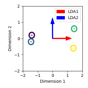
Because LDA-DR basically maximizes the pairwise squared distances between the whitened class means (see this StackExchange answer for a proof), the first LDA feature captures the large distance between the two pairs of classes. This direction is not very discriminative, since each class will have close to chance performance with respect to the overlapping class. The second LDA feature will have smaller distances between classes, but the classes will be more discriminable. Let’s visualize this by plotting the Gaussian densities of each class as projected onto the LDA features:

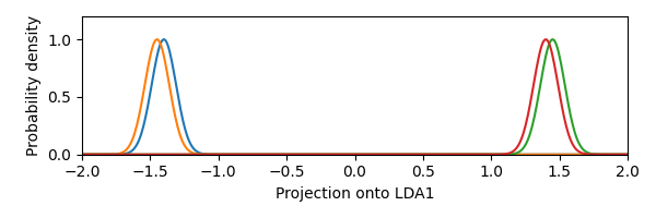
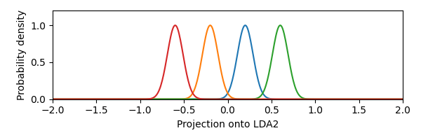
We see that the first LDA feature is not the most discriminative one. Thus, this example shows that the LDA-DR features do not necessarily maximize the performance of the LDA classifier, even if the classes satisfy the assumptions of the LDA classifier.

Information geometry interpretation of LDA

The objective of LDA can also be interpreted in terms of information geometry, which is the field that studies manifolds of probability distributions. If you are interested in learning more about this interpretation, check out my preprint “Supervised Quadratic Feature Analysis: An Information Geometry Approach to Dimensionality Reduction”.