
Easy constrained optimization in Pytorch with Parametrizations
Published:
Often times, we want to optimize some model parameter while keeping it constrained. For example, we might want a parameter vector to have unit norm, a set of vectors to be orthogonal with respect to each other, or a matrix to be symmetric positive definite (SPD). For the specific cases where the constraint is for the parameter to be on a manifold, a common approach is to use Riemannian optimization. However, there is a simpler and often more efficient way to do constrained optimization: we can use a technique called parametrization.
Parametrizations are a tool to turn a constrained optimization problem into a simpler unconstrained optimization problem. In this post we introduce parametrizations and show how to implement them in Pytorch. We will study two examples with synthetic data: constraining a vector to have unit norm, and constraining a matrix to be SPD.
We assume familiarity with PyTorch and basic optimization. More in depth information on Pytorch parametrizations can be found in the Parametrizations tutorial (aimed at more advanced users).
Constrained optimization
When doing optimization in Pytorch, we usually have a parameter \(\theta \in \mathbb{R}^n\) and a loss function \(L(\theta)\) that we minimize with gradient descent. For this, at each iteration we update \(\theta\) in the direction of the negative gradient of \(L(\theta)\):
\[\theta \leftarrow \theta - \alpha \nabla_{\theta} L(\theta)\]\(\nabla_{\theta} L(\theta)\) is the gradient of the loss function with respect to \(\theta\) and \(\alpha\) is the learning rate.
In constrained optimization, we also want to constrain \(\theta\) to fulfill some condition, or equivalently, to be in a certain subset \(C \subseteq \mathbb{R}^n\). One simple example is constraining a vector \(\theta\) such that \(\|\theta\| = 1\), or such that \(\theta \in C\), where \(C\) is the unit sphere \(C = \{x: \|x \| = 1\}\).
When we introduce a constraint, we can no longer just updating the parameter \(\theta\) in the direction of the negative gradient. Doing so is likely to break the constraint, e.g. it will drive \(\theta\) outside of the unit sphere \(C\). So, how can we update the parameter in such a way that it remains on \(C\)?
For the example of the sphere, an intuitive alternative is to project \(\theta\) back onto the unit circle by \(\theta \leftarrow \theta / \| \theta \|\) after each update. However, doing this naively can introduce problems. Also, while projecting onto the circle is straightforward, projecting onto other constraint sets (e.g. orthonormal vectors) might be more difficult.
There are different approaches to constrained optimization. Among these, parametrizations are a simple and efficient method that is easy to implement and that is popular in machine learning.
Formalism of parametrizations
Parametrizations involve projecting onto the set \(C\), but in a more principled way than the example above. The idea is to introduce a new unconstrained parameter \(\eta \in \mathbb{R}^m\), and a differentiable and surjective function \(f(\eta) = \theta\) that maps from values in \(\mathbb{R}^m\) to \(C\), \(f: \mathbb{R}^m \rightarrow C\). Then, we do optimization on \(\eta\) instead of \(\theta\), as follows:
\[\eta \leftarrow \eta - \alpha \nabla_{\eta} L\left(f(\eta)\right)\]We use the same loss function as before, but now composed with the function \(f\) so it is a function of \(\eta\). And we now take the gradient with respect to \(\eta\). Because \(\eta\) is unconstrained, we can update it with gradient descent, taking advantage of the highly efficient routines implemented for unconstrained optimization in Pytorch. The parameter of interest \(\theta\) is given by \(f(\eta)\) and it will always satisfy the constraint.
For our example of constraining \(\theta\) to be on the unit circle, we can parametrize \(\theta\) with the function \(f(\eta) = \eta / \| \eta \|\)1.
Lets see how we can implement this idea in Pytorch.
Example: Average on a circle, unconstrained
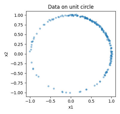
First, introduce a simple problem to illustrate constrained optimization: Finding the average of a set of points on the unit circle.
For this, we will have some data vectors \(x_i\) distributed in the unit circle, and we want to find the vector \(\theta\) that minimizes the squared distance to the data \(L(\theta) = \sum_i \| \theta - x_i \|^2\). We also want \(\theta\) to be on the circle.
Before showing how to solve the constrained optimization problem, lets implement the unconstrained optimization problem to use as a reference.
First we generate the data on the circle by sampling points from the distribution \(\mathcal{N}(\mu, \mathbb{I}\sigma^2)\) in \(\mathbb{R}^2\), and dividing these points by their norm 2.
### GENERATE THE DATA ON THE CIRCLE
import torch

# Simulation parameters
n_dimensions = torch.tensor(2)
mu = torch.ones(n_dimensions) / torch.sqrt(n_dimensions)
sigma = 1
n_points = 200

# Generate Gaussian data
data_gauss = mu + torch.randn(n_points, n_dimensions) * sigma
# Project to the unit sphere
data = data_gauss / data_gauss.norm(dim=1, keepdim=True)
We visualize the data
### PLOT THE DATA
import matplotlib.pyplot as plt

def plot_circle_data(ax, data, title):
    ax.scatter(data[:, 0], data[:, 1], alpha=0.4, s=12)
    ax.set_xlim(-1.1, 1.1)
    ax.set_ylim(-1.1, 1.1)
    ax.set_xlabel("x1")
    ax.set_ylabel("x2")
    ax.set_title(title)

data_jitter = data + 0.01 * torch.randn(n_points, 2)

fig, ax = plt.subplots(figsize=(4, 3.8))
plot_circle_data(ax, data_jitter, "Data on unit circle")
plt.tight_layout()
plt.show()
Next, we generate the Python class to perform the optimization. Our class AverageUnconstrained has parameter vector theta, and a function forward that computes the squared distance of each point to theta3. We use the Pytorch nn.Module class to define the model 4.
### DEFINE CLASS FOR UNCONSTRAINED OPTIMIZATION
import torch.nn as nn

class AverageUnconstrained(nn.Module):
    def __init__(self, dim):
        super().__init__()
        # Initialize theta randomly
        theta = torch.randn(dim)
        theta = theta / torch.norm(theta)
        # Make theta a parameter so it is optimized by Pytorch
        self.theta = nn.Parameter(theta)

    def forward(self, x):
        # Compute the distance of each point to theta
        difference = x - self.theta
        distance_squared = torch.sum(difference**2, dim=1)
        return distance_squared
Next, we define a function loss_function that computes the loss by taking the average of the squared distances. We also define the function train_model that performs gradient descent on the model parameters:
### DEFINE LOSS FUNCTION AND OPTIMIZATION FUNCTION
# Loss function
def loss_function(loss_vector):
    loss = torch.mean(loss_vector)
    return loss

# Optimization function
def train_model(model, data, n_iterations=100, lr=0.1):
    # We initialize an optimizer for the model parameters
    optimizer = torch.optim.Adam(model.parameters(), lr=lr)

    # We take n_iterations steps of gradient descent
    for i in range(n_iterations):
        optimizer.zero_grad()
        loss_vector = model(data)
        loss = loss_function(loss_vector)
        loss.backward()
        optimizer.step()
Lets use these functions to optimize the model and visualize the result.
### OPTIMIZE THE THETA AND VISUALIZE
# Initialize the model
model_unconstrained = AverageUnconstrained(n_dimensions)

# Fit the model
train_model(model_unconstrained, data, n_iterations=100, lr=0.1)

# Visualize the theta learned by the model
theta = model_unconstrained.theta.detach().numpy()

fig, ax = plt.subplots(figsize=(4, 3.8))
plot_circle_data(ax, data_jitter, "Unconstrained theta")
ax.scatter(theta[0], theta[1], color="red", s=20, label="theta")
ax.legend(loc="upper left")
plt.show()
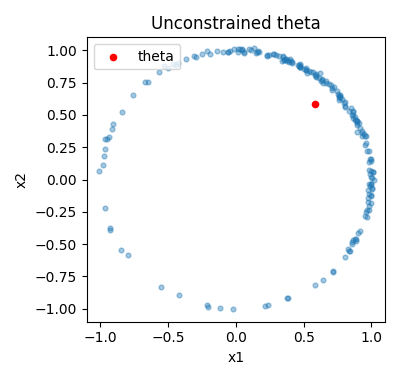
We see that the learned point is not on the circle, as we would expect since we did not add any constraint.
Implementation of unit circle constrain in Pytorch
We now implement a model that does constrained optimization using parametrizations. For this, we will use the Pytorch tool torch.nn.utils.parametrize, which takes care of a lot of the software bookkeeping for us, and can be implemented with minimal changes to our original code.
How to implement \(f\) for Pytorch parametrizations
To use parametrize, we need to define the function \(f\) inside an nn.Module class, implemented in the method forward inside this class. Let’s see how this looks like in our example:
# Define the parametrization function f
class NormalizeVector(nn.Module):
    def forward(self, eta):
        theta = eta / eta.norm()
        return theta
The method forward implements \(f\) by taking vector eta and returning the normalized vector theta with a length of 1 (the names of the variables don’t have to be eta and theta).
Next, let’s use parametrize to create a new class where theta is constrained to be on the unit circle. This is done by adding only one line to our original unconstrained class:
### DEFINE CLASS FOR CONSTRAINED OPTIMIZATION
from torch.nn.utils import parametrize

class AverageInCircle(nn.Module):
    def __init__(self, dim):
        super().__init__()
        # Initialize theta randomly
        theta = torch.randn(dim)
        theta = theta / torch.norm(theta)
        # Make theta a parameter so it is optimized by Pytorch
        self.theta = nn.Parameter(theta)

        ### ONLY CHANGE: Add the parametrization in terms of f to theta
        parametrize.register_parametrization(self, "theta", NormalizeVector())


    def forward(self, x):
        # Compute the distance of each point to theta
        difference = x - self.theta
        distance_squared = torch.sum(difference**2, dim=1)
        return distance_squared
Now, the unconstrained eta parameter that is actually being updated by gradient descent is taken care of in the background. Importantly, the code for optimizing the constrained model doesn’t change. Let’s optimize the model and see the result.
### OPTIMIZE THE CONSTRAINED THETA AND VISUALIZE
# Initialize the model
model_circle = AverageInCircle(n_dimensions)

# Fit the model
train_model(model_circle, data, n_iterations=100, lr=0.1)

# Visualize the theta learned by the model
theta_circle = model_circle.theta.detach()

fig, ax = plt.subplots(figsize=(4, 3.8))
plot_circle_data(ax, data_jitter, "Parametrized theta")
ax.scatter(theta_circle[0], theta_circle[1], color="red", s=20, label="theta")
ax.legend(loc="upper left")
plt.show()
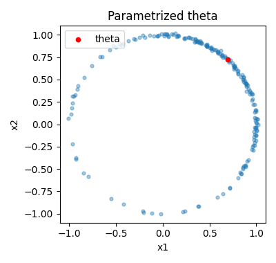
Now in this parametrized model the optimized theta is on the unit circle.
Implementation of symmetric positive definite parametrization in Pytorch
Let’s look at a more complicated example that appears often in statistics and machine learning: optimization of a matrix constrained to be SPD5. This is a common problem because covariance matrices and many other important mathematical objects are SPD matrices.
There are some well-known parametrizations for SPD matrices, and we will show how to implement two of them in Pytorch: the Log-Cholesky parametrization, and the matrix logarithm parametrization (see the article Unconstrained parametrizations for variance-covariance matrices for an overview).
Remember, to define a parametrization we need to define a function \(f\) that maps from the unconstrained parameter space to the space of SPD matrices. So, what we will do below is describe functions \(f\) that map from the unconstrained space of lower-triangular matrices (for the Log-Cholesky parametrization) and symmetric matrices (for the matrix logarithm parametrization) to the space of SPD matrices.
Log-Cholesky parametrization
The Log-Cholesky parametrization uses the property of SPD matrices that they can be decomposed as \(\Sigma = LL^T\), where \(L\) is a lower triangular matrix with positive diagonal elements (in this section we refer to our model parameter as \(\Sigma\) instead of \(\theta\)). This is called the Cholesky decomposition of \(\Sigma\), and it is unique.
A parametrization in terms of \(L\) though would not work, because \(L\) is constrained to have positive diagonal elements. The Log-Cholesky parametrization gets rid of this constraint by taking the logarithm of the diagonal elements of \(L\), resulting in an unconstrained lower-triangular matrix \(M\). Let’s see how we can define an \(f(M)=\Sigma\) according to this reasoning.
Let \(\lfloor M \rfloor\) denote the matrix with only the strictly lower-triangular part of lower-triangular matrix \(M\), and \(\mathbb{D}(M)\) the diagonal matrix with the diagonal elements of \(M\). Then,
\[M = \mathbb{D}(M) + \lfloor M \rfloor\] \[L = e^{\mathbb{D}(M)} + \lfloor M \rfloor\](note that to take the exponential of a diagonal matrix we just take the exponential of the diagonal elements). Then, the function \(f\) that maps from the unconstrained space of lower triangular matrices \(\mathbb{R}^{\frac{n(n+1)}{2}}\)6 to the SPD matrices is defined as follows:
\[f(M) = \left[ e^{\mathbb{D}(M)} + \lfloor M \rfloor \right] \left[ e^{\mathbb{D}(M)} + \lfloor M \rfloor \right]^T = L L^T = \Sigma\]Thus, we have a function that we can use to define our parametrization in terms of unconstrained parameter \(M\).
Before we implement this in Pytorch, we should note that there is one thing that parametrize needs some more help with: assigning specific values to the parameter \(\Sigma\).
Right-inverse function for assigning the constrained parameter
Suppose that we want to assign a specific value \(\Sigma'\) to the parameter \(\Sigma\), in our parametrized Pytorch model (e.g. we want to initialize it in a certain way). But in the parametrized model, there is a parameter \(M\) in the background that gives us \(\Sigma\) by \(f(M) = \Sigma\). Thus, we can’t just assign a value \(\Sigma'\) to \(\Sigma\), we need to assign a value \(M'\) to \(M\) such that \(f(M') = \Sigma'\). The parametrize tool takes care of the details of this, but it needs to be given a function that maps from \(\Sigma\) to \(M\), which is called right-inverse in the class with function \(f\).
We already described the right-inverse function for our Log-Cholesky parametrization when we explained how to get \(M\) from \(\Sigma\): 1) Take the Cholesky decomposition of \(\Sigma\) to get \(L\) 2) Take the logarithm of the diagonal elements of \(L\) to get \(M\)
Let’s now implement both the parametrization function \(f\) and the right-inverse function for the Log-Cholesky parametrization in Pytorch:
### IMPLEMENTATION OF LOG-CHOLESKY PARAMETRIZATION

# Log-Cholesky parametrization
class SPDLogCholesky(nn.Module):
    def forward(self, M):
        # Take strictly lower triangular matrix
        M_strict = M.tril(diagonal=-1)
        # Make matrix with exponentiated diagonal
        D = M.diag()
        # Make the Cholesky decomposition matrix
        L = M_strict + torch.diag(torch.exp(D))
        # Invert the Cholesky decomposition
        Sigma = torch.matmul(L, L.t())
        return Sigma

    def right_inverse(self, Sigma):
        # Compute the Cholesky decomposition
        L = torch.linalg.cholesky(Sigma)
        # Take strictly lower triangular matrix
        M_strict = L.tril(diagonal=-1)
        # Take the logarithm of the diagonal
        D = torch.diag(torch.log(L.diag()))
        # Return the log-Cholesky parametrization
        M = M_strict + D
        return M
We are now ready to implement a model that optimizes a matrix while constraining it to be SPD, using the Log-Cholesky parametrization. Let’s set up a problem to test this optimization.
Estimating a covariance matrix with missing data
We will use a problem suggested by a user at CrossValidated. The problem is estimating the covariance matrix of a dataset where some observations are missing, which is a common problem with real-world datasets.
We have a dataset \(X\) with \(n\) rows and \(p\) columns, where each row is an observation and each column is a variable. The dataset is missing some entries \(X_{ij}\) completely at random. The problem is that we want to estimate the covariance matrix of \(X\), which we call \(\Sigma\).
To estimate any given element \(\Sigma_{kl}\), we could use only the rows of \(X\) where both columns \(k\) and \(l\) are observed. However, this procedure does not guarantee that the resulting matrix is SPD. To solve this problem, we will do maximum-likelihood estimation of the covariance, ignoring the missing values. We will implement models to optimize \(\Sigma\) both without constraint and with the Log-Cholesky parametrization, and compare the results.
First, we generate a dataset for this problem. We start by generating a mean mu_true and a covariance matrix Sigma_true (we use our already defined \(f\) function to generate a random Sigma_true from a random M)
### GENERATE DATA PARAMETERS

# Set random seed
torch.manual_seed(1911)

# Generate the distribution parameters
n_dimensions = torch.tensor(5)
mu_true = torch.ones(n_dimensions)
M = torch.randn(n_dimensions, n_dimensions) / 10
log_chol_par = SPDLogCholesky()
Sigma_true = log_chol_par.forward(M)
Next, we generate the data by sampling from \(\mathcal{N}(\mu_{\text{true}}, \Sigma_{\text{true}})\), and setting some entries to be missing at random.
### GENERATE GAUSSIAN DATA WITH MISSING VALUES

from torch.distributions import MultivariateNormal

# Generate data
n_points = 200
data = MultivariateNormal(mu_true, Sigma_true).sample((n_points,))

# Remove random datapoints
mask = torch.rand(n_points, n_dimensions) > 0.2
# Make data where mask is False NaN
data[~mask] = float("nan")

# Print the first 8 rows of the data
print(data[:8])
tensor([[ 1.1146,  0.4793,  1.4138,  0.7827,     nan],
        [-0.9918,     nan,  0.4070,  1.7971,  1.4161],
        [ 1.3888,  1.8095,  0.9842,  0.4521, -1.9231],
        [ 0.9323, -0.0999,     nan,     nan, -0.9474],
        [ 2.3576,  1.7566,     nan,  0.3555,  0.7441],
        [ 1.8579,  1.3301,  1.1172, -0.0374,  2.5136],
        [ 1.0750,  1.2708,     nan, -0.4027,     nan],
        [ 0.7755,  2.7918,  1.0426,  1.2220,     nan]])
Next, we implement models that compute the negative log-likelihood of the data under a Gaussian distribution with parameters mu and Sigma, while ignoring missing values.
For a given data point \(x_i\) with missing values, we compute the log-likelihood of the observed values by using only the corresponding elements of mu and Sigma. That is, if a row has missing values for the columns \(1\) and \(3\), we will remove the elements \(1\) and \(3\) from the mu and the rows and columns \(1\) and \(3\) from the Sigma, and we will use the remaining elements to compute the log-likelihood with a Gaussian distribution of lower dimension.
We first implement three useful functions: gaussian_log_likelihood computes the log-likelihood of a data point under a Gaussian distribution, remove_nan_statistics takes as input the statistics mu and Sigma and returns the statistics with only the elements corresponding to the observed data, and nll_observed_data computes the negative log-likelihood of the dataset with missing values as described in the previous paragraph.
### IMPLEMENT FUNCTIONS TO COMPUTE MISSING DATA LOG-LIKELIHOOD

def gaussian_log_likelihood(data, mu, Sigma):
    # Compute the log likelihood of a single
    # data point under a Gaussian distribution
    n_dimensions = data.shape[0]
    # Subtract the mean from the data
    diff = data - mu
    # Compute the quadratic term
    quadratic = torch.einsum('i,ij,j->', diff, Sigma.inverse(), diff)
    # Compute the gaussian log-likelihood
    log_likelihood = -0.5 * (n_dimensions * torch.log(torch.tensor(2.0 * torch.pi)) \
                             + torch.slogdet(Sigma)[1] \
                             + quadratic)
    return log_likelihood


def remove_nan_statistics(mu, Sigma, nan_indices):
    # Remove the missing value elements from the mean and covariance
    mu_no_nan = mu[~nan_indices]
    Sigma_no_nan = Sigma[~nan_indices][:, ~nan_indices]
    return mu_no_nan, Sigma_no_nan


def nll_observed_data(mu, Sigma, data):
    # Compute the negative log-likelihood of the data under the
    # Gaussian distribution, ignoring NaN values
    ll = torch.zeros(data.shape[0])
    for i in range(data.shape[0]):
        # Get NaN indices for this row
        nan_indices = torch.isnan(data[i])
        # Remove the NaN columns from the statistics
        mu_no_nan, Sigma_no_nan = remove_nan_statistics(mu,
                                                        Sigma,
                                                        nan_indices)
        # Remove NaN columns from the data
        data_no_nan = data[i][~nan_indices]
        # Compute the likelihood of the observed data
        ll[i] = gaussian_log_likelihood(data_no_nan,
                                        mu_no_nan,
                                        Sigma_no_nan)
    return -ll
Now, we implement the model that computes the negative log-likelihood as described above, and we don’t constrain Sigma to be SPD:
### IMPLEMENT UNCONSTRAINED MODEL TO COMPUTE MISSING DATA NEGATIVE LL

class NLLObserved(nn.Module):
    def __init__(self, mu, Sigma):
        super().__init__()
        self.mu = nn.Parameter(mu.clone())
        self.Sigma = nn.Parameter(Sigma.clone())

    def forward(self, data):
        nll = nll_observed_data(self.mu, self.Sigma, data)
        return nll
We then implement the model that uses the Log-Cholesky parametrization, which only requires adding one line to the previous model:
### IMPLEMENT LOG-CHOLESKY MODEL TO COMPUTE MISSING DATA NEGATIVE LL

class NLLObservedCholesky(nn.Module):
    def __init__(self, mu, Sigma):
        super().__init__()
        self.mu = nn.Parameter(mu.clone())
        self.Sigma = nn.Parameter(Sigma.clone())

        ### ONLY CHANGE: Add the parametrization in terms of f to Sigma
        parametrize.register_parametrization(self, "Sigma", SPDLogCholesky())

    def forward(self, data):
        nll = nll_observed_data(self.mu, self.Sigma, data)
        return nll
We are now ready to optimize the models and compare the results. Because of how we set up the functions, we can use the same train_model function as in the previous example.
### OPTIMIZE THE MODELS

# Generate initial parameters
mu_init = torch.zeros(n_dimensions)
Sigma_init = torch.eye(n_dimensions)

# Initialize the models
model_unconstrained = NLLObserved(mu_init, Sigma_init)
model_cholesky = NLLObservedCholesky(mu_init, Sigma_init)

# Fit the models
train_model(model_unconstrained, data, n_iterations=100, lr=0.1)
train_model(model_cholesky, data, n_iterations=100, lr=0.1)
Let’s first check whether the covariance matrices are SPD for each model:
### CHECK IF COVARIANCE MATRICES ARE SPD

eigenvalues_unconstrained = torch.linalg.eigh(model_unconstrained.Sigma.detach())
eigenvalues_cholesky = torch.linalg.eigh(model_cholesky.Sigma.detach())

print("Minimum eigenvalue unconstrained model:", eigenvalues_unconstrained[0].min())
print("Minimum eigenvalue Cholesky model:", eigenvalues_cholesky[0].min())
Minimum eigenvalue unconstrained model: tensor(-3.0754)
Minimum eigenvalue Cholesky model: tensor(0.4976)
The covariance matrix of the unconstrained model is not positive definite, while the covariance matrix of the Log-Cholesky parametrized model is positive definite. Let’s see how the estimated covariances compare to the true covariance matrix:
### VISUALIZE THE LEARNED COVARIANCE MATRICES

# Visualize the learned Sigmas
fig, ax = plt.subplots(1, 3, figsize=(9, 3))

vmax = torch.max(torch.abs(Sigma_true))
vmin = -vmax

# True Sigma
im0=ax[0].imshow(Sigma_true, cmap="coolwarm", vmin=vmin, vmax=vmax)
ax[0].set_title(r"True $\Sigma$")
# Learned Sigma
ax[1].imshow(model_unconstrained.Sigma.detach(), cmap="coolwarm", vmin=vmin, vmax=vmax)
ax[1].set_title(r"Unconstrained $\Sigma$")
# Learned Sigma with Cholesky parametrization
ax[2].imshow(model_cholesky.Sigma.detach(), cmap="coolwarm", vmin=vmin, vmax=vmax)
ax[2].set_title(r"Log-Cholesky parametrized $\Sigma$")
# Add a colorbar to the right of the subplots
cbar = fig.colorbar(im0, ax=ax.ravel().tolist(), shrink=0.95,
                    cax=plt.axes([0.93, 0.15, 0.02, 0.7]))

plt.show()
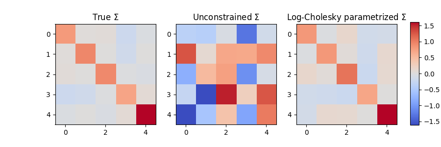
We see that not only is the covariance matrix of the constrained model positive definite, but it is also much closer to the true covariance matrix than the unconstrained model!
Matrix logarithm parametrization
That’s all we are going to show about parametrizations, but we want to show one more example of a parametrization, since everyone loves parametrizations of SPD matrices. We will not go into detail on this parametrization, or use it to solve our problem, but just show how to implement it in Pytorch.
The logarithm and exponential of a matrix are defined in terms of series of matrix powers. For invertible matrices however (like SPD matrices), the matrix logarithm and exponential can be obtained as \(\log(A) = U \log(\Lambda) U^{-1}\) and \(\exp(A) = U \exp(\Lambda) U^{-1}\), where \(A = U \Lambda U^{-1}\). For a given SPD matrix, we obtain the matrix logarithm by taking the eigenvalue decomposition, taking the logarithm of the eigenvalues, and then reconstructing the matrix.
While an SPD matrix has positive eigenvalues, its matrix logarithm can have any real eigenvalues. In fact, the matrix logarithm of an SPD matrix will be a symmetric matrix. Thus, the matrix logarithm function maps from the SPD matrices space to the simple vector space of symmetric matrices. Conversely, the matrix exponential maps from the symmetric matrices to the non-linear space of SPD matrices.
From the above, we see that we can parametrize SPD matrices in terms of the unconstrained space of the lower-triangular part of symmetric matrices, with \(f\) being the matrix exponential, and its right-inverse being the matrix logarithm. Let’s implement this in Pytorch:
### IMPLEMENTATION OF MATRIX LOGARITHM PARAMETRIZATION

import scipy # Scipy has the matrix logarithm function

# Define positive scalar constraint
def symmetric(X):
    # Use upper triangular part to construct symmetric matrix
    return X.triu() + X.triu(1).transpose(0, 1)

class SPDMatrixExp(nn.Module):
    def forward(self, X):
        # Make symmetric matrix and exponentiate
        SPD = torch.linalg.matrix_exp(symmetric(X))
        return SPD

    def right_inverse(self, SPD):
        # Take logarithm of matrix
        symmetric = scipy.linalg.logm(SPD.numpy())
        X = torch.triu(torch.tensor(symmetric))
        X = torch.as_tensor(X, dtype=dtype)
        return X
Optimization on manifolds
Many constrained optimization problems can be seen as optimization on manifolds, particularly matrix manifolds. The sphere and the SPD matrices examples we showed are examples of manifolds. The reader interested in other examples of how to use parametrizations for constrained optimization can check the package geotorch for optimization in manifolds, which implements several parametrizations for manifolds in Pytorch. Curiously, the developer of geotorch, Mario Lezcano, is the same person who developed the Pytorch parametrizations tool we used in this post, and who wrote the Parametrizations tutorial in the Pytorch documentation. Thank you Mario for making time to chat about manifolds with me!
Note that actually, the function \(f(\eta) = \eta/ \| \eta \|\) does not map from \(\mathbb{R}^m\) to the unit circle, because it is not defined at 0. However, in practice this is not generally a problem, as $\eta$ will not generally be driven towards 0 in this setup. ↩
Of interest, the distribution on the sphere obtained by projecting a Gaussian distribution is known as the Angular Gaussian or Projected Normal distribution. ↩
Functions named
forwardare called when we call the call the model object as a function, i.e.model(data)↩A Pytorch
nn.Moduleis a Pytorch class that has several methods that are useful for defining and optimizing models. By creating our class with the callclass MyClass(nn.Module):, the class inherits these methods fromnn.Module. These then come in handy for example to define parameters withnn.Parameter, or to pass the model to an optimizer. ↩SPD matrices are symmetric matrices whose eigenvalues are all positive. There is no simple condition on the matrix entries to ensure that it is SPD. ↩
Note that although \(M\) is a matrix, it is equivalent to an unconstrained vector in \(\mathbb{R}^{\frac{n(n+1)}{2}}\) having its lower-triangular elements, and it is unconstrained ↩